Snakes & ladders is a classic board game, originally imported into the United Kingdom from India circa 1890 according to Wikipedia. Its a square grid numbered row wise from 1-100, with some of the cells connected together either by a snake or a ladder. Players roll a dice and then advance that many steps. If a player lands on the head of a snake or the foot of a ladder they are transported to the respective other end. The objective is to get to or (past) the last cell.
I was playing Snakes & Ladders the other day which is a very boring game to play since it involves no decision making at all. To pass the time I started noodling on how I’d calculate how many turns a game is expected to take, which is what you’ll find herein.
For simplicity, but without loss of generality, we can use a smaller board (say \(4 \times 4\)) and a dice with fewer than 6 sides (say \(3\)): it makes the problem easier to write down and diagrams easier to draw. Here is an example board with the arrows indicating snakes/ladders based on their effect.

A practical analysis
We can analyse this as a graph problem, so lets start by building a matrix \(P\) to take into account both which transitions are possible and how probably they are given our 3 sided dice: \(P_{i,j}\) indicates the probability of transitioning from cell \(i\) to \(j\). The board above would imply a \(16 \times 16\) matrix, so even for small boards writing out the transitions by hand is impractical, and it is more convenient to calculate the matrix algorithmically:
t_matrix <- function(N,M) {
  N  <- N^2
  Cs <- seq(1:N)
  Ss <- c(2,8,10,14)
  Es <- c(7,3,13,5)
  X  <- outer(Cs, Cs, Vectorize(\(i,j) {
    cond1 <- j > i && !(j %in% Ss) && i+M >= j
    k <- which(Es==j)
    cond2 <- length(k) > 0 && i < Ss[k] && i+M >= Ss[k]
    ifelse(cond1 || cond2, 1, 0)
  }))
  X[(N-M):N,N] <- X[(N-M):N,N] * seq(1,M+1) # Overrun adj.
  X
}

T <- t_matrix(4,3)
X <- 1/rowSums(T)
P <- T * ifelse(is.finite(X), X, 0)
Since the transitions are independent, we can get the probability of any particular \(n\) step path by walking through a set of connected transitions and multiplying their probabilities. By the same merit, from Markov theory, we can get the probability of all \(n\) step transitions between every pair of cells from the power matrix \(P^n\).
All that remains is to create a profile for transitioning from cell \(1\) to \(16\), in \(n\) turns, and then calculate the expected value and a CDF in the usual way.
n <- seq(1,70)
x <- sapply(n, \(n) (P %^% n)[1,16])
mu <- sum(n * x)
plot(n, cumsum(x), main=paste("E(n) =", round(mu)),
type="l", xlab="n", ylab="p")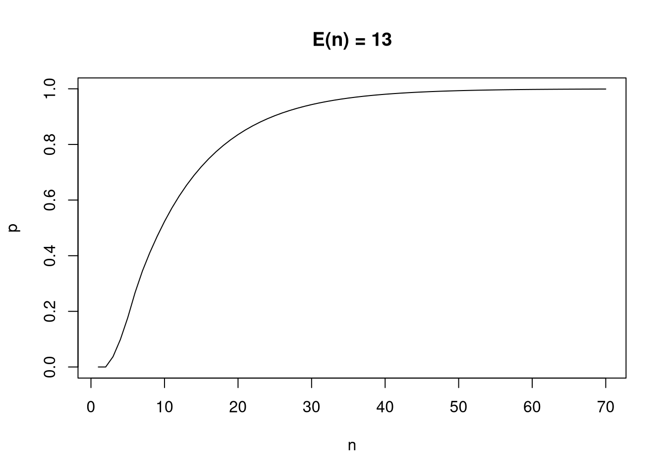 The maximum probability of the CDF is 0.999 – a close
approximation – and from it we can easily calculate other useful information
such as confidence intervals and tail probabilities.
The maximum probability of the CDF is 0.999 – a close
approximation – and from it we can easily calculate other useful information
such as confidence intervals and tail probabilities.
Closed form expectation
The above method is intuitive and possibly the easiest for calculating a CDF, but with a little bit of additional Markov theory we can calculate the expected number of rolls in closed form.
Let’s quickly derive the hitting time formula because its straightforward. Say we want \(h_i\) – the number of turns required to reach the last cell \(n\). from cell \(i\). We must take at least \(1\) turn, at which point we are either at \(n\) or in some other cell \(j\). From \(j\) the number of turns required is \(h_j\). Since we do not know which cell \(j\) we will land on, we average over the possibilities. In our case we’d like to transition from cell 1 to 16, and therefore we are interested in: \[ h_1 = 1 + P_{1,2} h_2 + P_{1,3} h_3 + \dots + P_{1,15} h_{15} \] Note cell 16 is not featured since \(h_{16}\) is zero. We can easily write this equation out for all \(h_i\), stack them, and express it in matrix form to get: \(h = \mathbf{1} + Qh\) where \(Q\) is just \(P\) with the row and column of the target cell \(n\) removed. We can now solve for \(h\), and read off the value at \(h_1\). That is: \[ h = (1-Q)^{-1}\mathbf{1} \] Beautiful and surprising. Here is an implementation in a line of code:
h <- solve(diag(15) - P[-16, -16], rep(1, 15))
print(paste("E[n] =", round(h[1])))
## [1] "E[n] = 13"as required.