Here are a few practical questions of my own invention which are easy to comprehend but very difficult to solve without statistical reasoning competence. They are provided in order of difficulty. The answers are at the end. If you find errors or have elegant alternative solutions, please email me (address in bio)!
QUESTIONS
1. Sorting fractions under uncertainty
You are given the number of trials and successes for a set of items, and you are asked to sort them by the fraction #successes / #trials. However, it is very important that the uncertainty in the number of trials is taken into account because over-estimating a fraction is a costly mistake.
Here is some example data.
| Item | Successes | Trials |
|---|---|---|
| 1 | 3 | 4 |
| 2 | 20 | 40 |
| 3 | 5 | 10 |
| 4 | 7 | 9 |
| 5 | 50 | 70 |
Order the items above, smallest fraction first, whilst taking into account the sample size uncertainty (number of trials) to bound the probability of over-estimating each fraction. Carefully explain your approach.
2. Highlighting unexpected domestic burglaries
You are given a map divided into grid cells. For each cell you are given a count of domestic burglaries in that area. You can request any other information about the cells which you might want. You are asked to find the top \(k\) most unexpected cells in terms of domestic burglary numbers. Carefully explain your approach.
3. Estimating the number of buses
You’ve decided to estimate the number of distinct buses with routes passing through your local bus stop. You do this by visiting the bus stop once every day, at a random time, writing down the license plate of the first bus you see, and leaving. You assume that your sampling strategy makes the probability of picking any given bus equal, and that the population of buses passing your bus stop remains the same through the sampling period.
After two weeks, you’ve collected the following data.
| License plate | Sightings |
|---|---|
| 1 | 1 |
| 2 | 1 |
| 3 | 2 |
| 4 | 2 |
| 5 | 1 |
| 6 | 1 |
| 7 | 3 |
| 8 | 1 |
| 9 | 2 |
Provide an interval estimate for the total number of buses passing through your local bus stop. Carefully explain your approach.
ANSWERS
1. Sorting fractions under uncertainty
Each fraction has to be modelled as a distribution in order take its uncertainty into account. The binomial distribution is a good choice, such that \(k \sim Binom(n,p)\) where \(k\) is the number of successes, \(n\) the number of trials and \(p\) the fraction of successful trials. We are given \(k\) and \(n\), but we are interested in the distribution of \(p\). There are many specific ways to produce a confidence interval for \(p\), the lower bound of which can be used to order the fractions, and so control the risk of over-estimation.
There are at least two general – from first principles – approaches to calculate a lower bound fraction without knowing specific formulae. The first – Bayesian – is to assign a prior to \(p\) and then take the \(q\) quantile of the posterior distribution as a lower bound estimate. One example of this is to use the beta distribution prior (closed form and conjugate of the binomial distribution) and then the posterior is given by \(p \sim beta(k+\alpha, n-k+\beta)\), where \(beta(\alpha, \beta)\) was your prior. In R:
# flat prior beta(0.5,0.5)
# 5th quantile for 3 successes and 4 trials.

qbeta(0.05, 3 + 0.5, 4-3+0.5)
## [1] 0.3492928The second – likelihoodist – is to create a profile likelihood and take the \(q\) quantile. I personally find this approach more intuitive in general because it is contextually picking model parameters, rather than to directly making claims about degrees of belief: we are just trying to pick \(p\) such that it captures the first 5% of the likelihood sum of our binomial model.
# 5th quantile profile likelihood for
# 3 successes and 4 trials.

fs <- seq(0,1,0.001)
ps <- sapply(fs, \(p) dbinom(3, 4, p))
ps <- cumsum(ps / sum(ps))
max(fs[ps <= 0.05])
## [1] 0.3422. Highlighting unexpected domestic burglaries
Lots of unsurprising factors will explain the number domestic burglaries in a cell such as the number of property related crimes more generally, the number of houses/apartments, average income, etc. You should realise that an “expected” count will be well modelled by the unsurprising factors and that an unexpected count will be a deviation from this model.
A simple approach – with assumptions about the variance – would be to assume the count is Poisson distributed and to model it as \(x \sim Poisson(\alpha X + \beta)\) where \(X\) is the factor matrix, and then to order the cells by \(p(X=x \mid \alpha, \beta)\) and take the top \(k\). A more advanced approach may be to use a continuous distribution (of which there are more choices) and to also model the variance prior to sorting by the probability.
3. Estimating the number of buses
It often helps to consider what the data generating distribution for a problem could be. In this case, some hidden \(k\) buses with the same chance of geting picked with a sample size of 14, is just like rolling a \(k\) sided dice 14 times and writing down how many times each side occurred: the multinomial distribution. We can simulate our situation by generating a count vector given \(n\) samples for \(k\) buses, and removing the zeros.
simulate <- \(k,n)
  rmultinom(1, n, rep(1/k, k)) %>%
    as.vector %>% .[. > 0]

# For k=10 buses
simulate(10, 14)
## [1] 1 1 2 2 2 1 2 1 2the complication here is that it does not help us to use the multinomial distribution on the resulting sample, because we cannot fix \(k\) and so do not know which “slot” each count should go in nor how many zero counts there are. However, it is not difficult to come up with a density function from first principles.
Assuming a fixed \(k\), let’s take as example the count vector \(x = (1,1,2)\). This implies that there are three slots in the multinomial with counts \(1,1,2\) respectively, and \(k - |x|\) slots with zero counts. Since we are assuming each slot is picked with equal probability every possible count for \(n\) samples has the same probability \((1/k)^n\). All that remains is to calculate how many possible arrangements would result in a count \(1,1,2\), which is just a matter of applying the multinomial coefficient. Say, \(k=7\), that would mean that two slots are allocated a \(1\), one slot is allocated a \(2\) and four slots are allocated \(0\): these are called “multiplicities”. So using the multinomial coefficient, that implies \(\frac{7!}{2!1!4!} = 105\) arrangements, all with probability \(p = (1/7)^4 \approx 0.0004\), and a final probability of \(105 \times p \approx 0.04373\). In the general case:
\[ p(x \mid k, n) = (1/k)^n \times \frac{k!}{m_1!..m_l!(|x|-k)!} \] where \(m_1...m_l\) are the multiplicities of the \(l\) non-zero counts.
In R:
P <- \(x, k) {
  f <- factorial
  l <- length(x)
  z <- ifelse(k-l <= 0, 0, k-l)
  (1/k)^sum(x) * f(k) / (prod(f(table(x))) * f(z))
}
Once we have a density function, all that remains is to fit \(k\), for which, as before, there are at least two first principle approaches. In the Bayesian approach you would either try to derive a closed-form prior (there might be one given the similarity to the multinomial distribution), or use some software such as nimble, Stan or PyMC3 to calculate the posterior of \(k\) given an arbitary prior of your choice. Alternatively – and demonstrated herein – you could calculate a likelihood profile and take a 95% confidence interval.
Since \(k\) is discrete, it should be bounded to something sensible for the problem. In the function below, I just calculate \(P\) for different values of \(k\), order them in probability descending order, and collect up to 95% of the mass to create an interval. Since the distribution is concave, this ordering procedure guarantees the confidence interval will both contiguous and the highest density interval possible.
# Using the sighting vector from the question.
x <- c(1,1,2,2,1,1,3,1,2)
# Upper bound for the number of buses.
K <- 100
ks <- length(x):K
y <- sapply(ks, \(k) P(x, k))
p <- y / sum(y)
ks <- ks[order(-p)]
p <- cumsum(p[order(-p)])
ks <- ks[p <= 0.95]
mn <- min(ks)
mx <- max(ks)
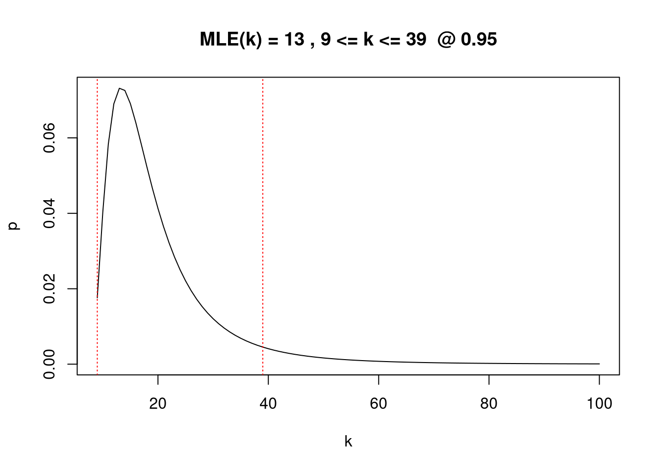
c(ks[1], mn, mx)## [1] 13 9 39It may help to plot it to see what’s going on:
plot(length(x):K, y/sum(y), type="l",xlab="k",ylab="p")
abline(v=mn, col="red", lty="dotted")
abline(v=mx, col="red", lty="dotted")
title(paste("MLE(k) =",ks[1],",",mn,"<= k <=",mx," @ 0.95"))