A basic application of linear methods are linear regression models. However, in some settings, they can be limiting at least because: (1) they may have few degrees of freedom and therefore saturate quickly, and (2) they may imply a rigid geometry (a hyper-plane) which is often unrealistic.
It turns out that if we can express similarity between data points as a Gram matrix, we can do linear regression directly to it; otherwise known as “Kernel” regression. The proverbial \(X\alpha = y + \epsilon\), solved using the OLS estimator \(\alpha = (X^\top X)^{-1}X^\top y\), becomes \(K\alpha = y + \epsilon\) where \(K\) is a \(m \times m\) Gram matrix (given \(m\) data points). \(K\) will likely be near-singular – since there are as many columns as rows – which we can alleviate by introducing the Ridge penalty to the OLS estimator such that: \(\alpha = (X^\top X + I\lambda)^{-1}X^\top y\), where \(\lambda \in \mathbb{R}\). Et voila, and in closed-form, we have enough machinery to perform so-called “Kernel Ridge regression”.
The radial basis kernel (RBF), \(K(x,x') = exp (-\gamma || x-x' || ^2)\), is a similarity measure based on an exponentially tapering squared Euclidean distance: \(\gamma\) decides how quickly it tapers. We can define the matrix \(K\) by calculating \(K(x,x')\) for every pair of data points, and fit it as above. The prediction function is then given by \(y_i = \alpha \cdot K(x_i, \cdot)\): note that the contribution of each component is weighted by (exponentially tapering) similarity to all other data points, which changes the geometry of the model dependent on its locality, thereby addressing the rigid geometry problem.
An issue with Kernel methods is that the space complexity is quadratic due to the \(m \times m\) Kernel matrix. One way to scale kernels to much bigger data is through kernel approximation by basis expansion. For the RBF kernel, an elegant such method is known as “random Fourier features”. It was introduced in a seminal paper which went on to win the NIPS 2017 test of time award.
The RBF kernel basis vectors are created by randomly sampling the Fourier transform of the kernel:
\[\phi(x) = \sqrt{\frac{2}{D}} \bigg[cos(g_1(x)),sin(g_1(x)), ..., cos(g_D(x)),sin(g_D(x))\bigg]\]
where \(g_i(x) = \omega_i^\top x+b_i\), and \(\omega_i, b_i\) are sampled \(D\) times, such that \(\omega_i \sim N(0,\gamma^{-1})\) and \(b_i \sim [0,2\pi]\). Note that the space complexity of the approximation is \(O(mD)\), so we are able to apply it to much bigger data.
Let’s give it a go in R. Here is a naive direct application to the Boston housing data. Nota bene however that in the general case, naively applying a Kernel on arbitrary explanatory vectors does not make sense. The Kernel needs to induce a meaningful similarity matrix, else the inferences from it will be nonsense.
require(mlbench, quietly=T)

data("BostonHousing")

X      <- BostonHousing[, -which(names(BostonHousing)=="medv")]
X$chas <- as.numeric(as.character(X$chas))
X      <- as.matrix(X)
y      <- matrix(BostonHousing$medv, ncol=1)
Here is the mean squared error between the response and a linear regression:
const  <- matrix(rep(1,NROW(X)), ncol=1)
X_     <- cbind(const, X)
beta   <- solve(t(X_) %*% X_) %*% t(X_) %*% y
y_     <- X_ %*% beta
lr_mse <- mean((y-y_)^2)  #cor(y,y_)
lr_mse
## [1] 21.89483Here is a routine to generate Fourier random features, fit them and test the mean squared error:
go <- function(D=200, gam=1, lam=0.1) {
W <- matrix(rnorm(D * NCOL(X), mean=0, sd=1/gam),
nrow=D)
B <- runif(D, min=0, max=2*pi)
X_ <- sweep(X %*% t(W), 2, B, "+")
X_ <- cbind(cos(X_), sin(X_)) / sqrt(2/D)
const <- matrix(rep(1,NROW(X)), ncol=1)
X_ <- cbind(const, X_)
I <- diag(ncol(X_))
beta <- solve(t(X_) %*% X_ + lam * I) %*% t(X_) %*% y
y_ <- X_ %*% beta
mean((y-y_)^2)
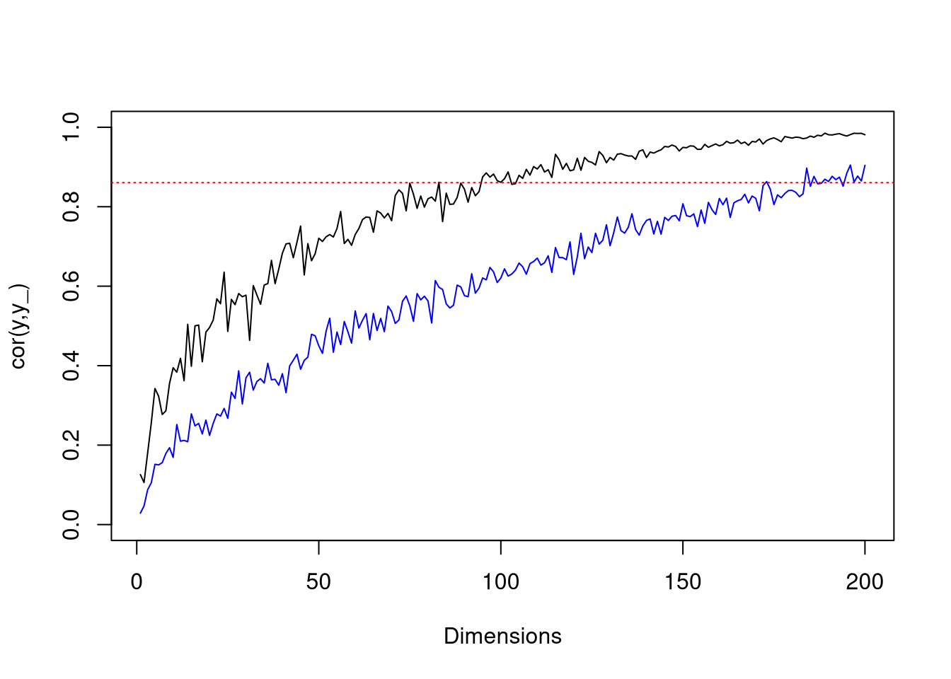
}Here are some plots to illustrate the effect of dimension on mean squared error, and and gamma on convergence (\(\gamma=12\) and \(\gamma=1\) for black and blue lines respectively). The dotted red line is the mean squared error achieved with linear regression.
plot  (
  sapply(1:200, \(i) go(i,gam=12)),
  pch=19, cex=0.25,  type="l",
  xlab="Dimensions", ylab="mse(y,y_)")

lines (
  sapply(1:200, \(i) go(i, gam=1)),
       pch=19, cex=0.25, col="blue")

abline(h=lr_mse, lty="dotted", col="red")