Introduction

I happened upon a post by Gwern discussing, in some detail, various solutions to riddle #14 from Nigel Coldwell’s list of quant riddles. I initially got as far as the problem description in Gwern’s article and avoided reading further so I could first solve it for myself. The problem is stated as follows:

You have 52 playing cards (26 red, 26 black). You draw cards
one by one. A red card pays you a dollar. A black one fines
you a dollar. You can stop any time you want. Cards are not
returned to the deck after being drawn. What is the optimal
stopping rule in terms of maximizing expected payoff? Also,
what is the expected payoff following this optimal rule?

I expected this problem to involve some kind of “statistical trick” so I started out with many unsuccessful forays only after which I started to examine it from first principles. Here are some fun dead ends:

What does the space over all possible stopping strategies look like?
Can I use the hyper-geometric distribution to calculate probabilities of different outcomes N steps ahead and then make a decision based on that?
Can I decide based on the total number of future sequences with a maximum total bigger than the current one?

In so far as getting maximum pedagogical value from a toy problem is concerned, I’m rather grateful I took such a roundabout route to the solution because it helped me “re-dial” my intuition towards analysis from an elementary point of view as a default. Once a problem is understood on that basis, it is much easier to correctly select tools and recast it into a tractable form, whilst initially assuming a tractable form runs risk of mischaracterising the problem and so failing to solve it.

Starting from first principles, it helps to pick a more minimal version of the problem – say 2 red and 2 black cards – and to draw out the possibilities as a tree. In the tree below, the nodes indicate the cumulative reward and the edge labels indicate the probabilities of the transition.

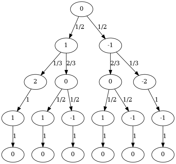
Given the diagram, I think it is natural to ask “how would I decide what to do at each node?”, and build up a stopping strategy from there. I should clearly stop at the node with a total of 2 because it can only get worse from there. Whenever the node total is less than or equal to zero, I should not stop since every sequence ends in a zero total anyway, so I cannot be worse-off. That leaves me only with nodes at a positive total where I have something to lose and must decide whether it is worth the risk or not. There is only “one show in town”, in terms of how to solve for this last case: some notion of expectation must come into play which can quantify the reward for not-stopping which I can compare it to the reward for stopping and thus make a decision. Note that such a notion would also likely deal with the cases where the reward is zero or less thus mitigating the need for a case based treatment.

The framing of the problem implies a uniform prior over the possible sequences of cards which are drawn without replacement, so there really is no patterns to match or other fancy footwork to draw on: I need to use a probability weighted average over the “reward” of each branch to calculate a statistical expectation. However, there is an apparent circularity here: calculating the “reward” for any given branch of a node implies I know how I’m going to decide further down the sequence. To see how to resolve this, let us take the left-most zero child node as an example wherein the possible future sequences are $(Red,Black)$ or $(Black,Red)$, each with a probability of 0.5. It is intuitive to me that I should consider the reward for the right branch to be zero but for the left branch to be 1 since if the left branch occurs I could stop early, whilst if the right branch occurs I could play-on. The calculation for the expectation should therefore be: $1\times 0.5 + 0\times 0.5 = 0.25$. This led me to understand that the reward at a node should be the greater of the expected reward for not stopping and the reward for stopping, since once at the node I can decide what to do, hence the reward for the zero node in the example as considered from the node above it should be $0.25$, not zero. Starting at the bottom of the tree, this process can be recursively applied to “roll up” the expectations from the bottom to the top, thus calculating the expected reward at the root (and every other) node before play begins. I can succinctly express this calculation as a Prolog programme:

:- table expect/4.

expect(0,_,Expect,Expect) :-!.
expect(R,0,Total,Expect) :-
    Expect is R + Total,!.
expect(R,B,Total,Expect) :-
    R>0,B>0,
    R0 is R-1,
    T0 is Total+1,
    expect(R0,B,T0,E1),
    B0 is B-1,
    T1 is Total-1,
    expect(R,B0,T1,E2),
    Sum is E1*R/(R+B) + E2*B/(R+B),
    Expect is max(Total, Sum).

The tree for riddle #14 is massive but its sub-trees repeat whenever the R, B and Total variables repeat, so the calculation can be performed many orders of magnitude faster by memoising the expect predicate. The Prolog equivalent to this is called “tabling” which in SWI-Prolog can be invoked using the table predicate as shown above. Finally, I can calculate the answer (and the time taken to execute the calculation) as follows:

?- time(expect(26,26,0,E)).                                                                                                    

% 29,164 inferences, 
% 0.003 CPU in 0.003 seconds (100% CPU, 10664915 Lips)                                                      
E = 2.6244755489939244.

The strategy yields an expectation of about $2.62. It is optimal because decisions happen sequentially and present decisions are unconditional on prior decisions. Therefore, if the expectation at the leaf nodes of the tree are correct, the expectations at their parent nodes will also be correct, and so on all the way up.

An optimal-stopping quant riddle

Introduction