Summary
I demonstrate a widely applicable pattern which integrates Prolog as a critical component in a data science analysis. Analytic methods are used to generate properties about the data under study and Prolog is used to reason about the data via the generated properties. The post includes some examples of piece-wise regression on timeseries data by symbolic reasoning. I also discuss the general pattern of application a bit.
Introduction
Given some data, the bulk of “data science” for me is the study of what the data implies and whether it can be coerced into the context specific role usually decided by someone other than me. Dependent on the context, the goal may be to find support for a hypothesis, to forecast, to predict a latent variable, to explain a phenomena, and so on. The majority of the value I bring rests in taking as input the data and the role it is expected to play, and producing as output a computationally tractable problem the solution to which enables that role for the data.
In my own practice – at least in its mature form – I find myself mostly relying on reasoning with simple methods such as Linear Regression, kNN, kMeans and PCA. I think this is mostly because I can understand what the results imply for the “shape” of the data, meanwhile reasoning about the results does the heavy lifting. Despite the importance of reasoning in my work, I never made it explicit, nor did I consciously separate it from its subject matter. When I became aware of this, it seemed to me that I should make my reasoning explicit at least so that I could (1) reason more accurately, and (2) directly learn to reason better.
It is easier to demonstrate what it means to make reasoning explicit and the effect it has on the structure of an analysis. What follows are a couple of illustrative examples. I use SWI Prolog as the symbolic reasoning engine and logic language, and Python for everything else.
A pedagogical example
I’ll start with a contrived example meant to illustrate the separation between the reasoning element and the rest. Below (black line) is some mock 2D data constructed by joining together 5 randomly selected lines into a series. The x-axis is just an index which runs from 0-999. The coloured segments are a piecewise linear fitting derived symbolically using Prolog. I’ll next describe how.
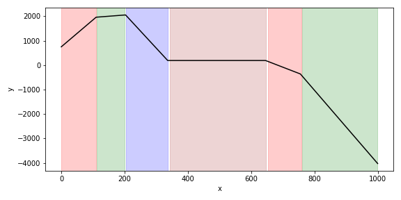
Say I do not know anything about the construction of the data series above except that it is made up of lines and the aim of the analysis is to find all the linear sections. My general scheme will be to use Python to create symbols which represent facts about the data, and then to use Prolog to reason about those symbols. One broadly applicable way of generating symbols is to partition the data at random along the explanatory variables (the \(x\) in this case) and fit linear regressions to each partition segment. This is then repeated many times in order to capture views of the data across many partitions. The result is lots of overlapping segments for which I can record information such as:
- Where the segment starts and ends.
- The fitting parameters.
- Correlation with the data.
Given some data \(X,Y\), the code below will produce rounds of random partitions (4-10) with segments at least 20 units wide, until there are at least \(N\) qualifying (perfectly linear) segments.
import numpy as np
from sklearn.linear_model import LinearRegression

i = 0
np.random.seed(10)
while i < N:
    knots = make_knots(
        np.random.randint(4,10),
        20,
        np.min(X),
        np.max(X))

    for start, stop in zip(knots[:-1], knots[1:]):
        cond = X[(X>=start) & (X<=stop)]
        x, y = X[cond].reshape(-1,1), Y[cond]
        m = LinearRegression().fit(x,y)
        p = m.predict(x)
        i += 1
        coef = np.round(m.coef_[0],4)
        score = m.score(x,y)
        if score ==1.0:
            print(f"segment(i{i},{start},{stop},{coef},{score}).")
Note that the code prints out strings in the following format:
segment(Id,Start,End,Gradient,Score).I copy/paste these directly into Prolog for demonstration purposes, but there are less manual ways.
The simple procedure above produces plenty of symbols to reason about. For example, segments may be separate, overlapping, subsuming, adjacent, etc. Gradients may be equal, similar, opposing, and so on. For these problems, I will only need to use a fraction of the information available. To produce the segmentation illustrated in the graph above, it is enough to note that if segments are perfectly linear and they overlap, then they must be the same line. I can use this assertion as a way of merging segments together in order to create bigger continuous linear spans. In Prolog I could express this as follows:
overlap(I1,I2) :-
    segment(I1,Start1,End1,_,_),
    segment(I2,Start2,End2,_,_),
    Start2 > Start1,
    End1 > Start2,
    End2 > End1.

:- table reach/2.

reach(I1,I2) :-
    overlap(I1,I2).
reach(I1,I2) :-
    overlap(I1,X),
    reach(X,I2).
That is to say, segment \(I1\) overlaps with segment \(I2\) if it begins outside of \(I2\) but ends inside of it. A segment \(I2\) can be “reached” from segment \(I1\) iff there is a daisy chain of overlapping segments connecting them. Based on the relationships above, the following query would produce all reachable spans (daisy chains of segments):
?- setof((I1,I2),reach(I1,I2),Spans).Prolog digression: overlap is intentionally non-commutative to prevent backtracking from looping. I use tabling on the reach predicate because SLD resolution is very inefficient in this case.
To calculate an optimal piece-wise linear fitting, I need to find the subset of all the non-overlapping spans generated by reach which result in the maximal coverage of the data. This can be as simple as sorting the spans by length in descending order and adding them to a list whilst making sure new additions do not overlap with the old ones. In Prolog:
use_module(library(apply)).
use_module(library(pairs)).

span_overlap((I1,I2),(I3,I4)) :-
    segment(I1,Start1,_,_,_),
    segment(I2,_,End1,_,_),
    segment(I3,Start2,_,_,_),
    segment(I4,_,End2,_,_),
    ((End1 >= Start2, End2 >= End1)
    ;(End2 >= Start1, End1 >= End2)
    ;(Start1 >= Start2, End2 >= Start1)
    ;(Start2 >= Start1, End1 >= Start2)).

not_span_overlap((I1,I2),(I3,I4)) :-
    \+ span_overlap((I1,I2),(I3,I4)).

span_length((I1,I2),R) :-
    segment(I1,Start,_,_,_),
    segment(I2,_,End,_,_),
    R is Start-End.

span_set([],R,R).
span_set([(X,Y)|T],A,R) :-
    maplist(not_span_overlap((X,Y)),A),
    (X=Y;reach(X,Y)),!,
    span_set(T,[(X,Y)|A],R).
span_set([_|T],A,R) :-
    span_set(T,A,R).

spans([],R,R).
spans([(I1,I2)|T],A,R):-
    segment(I1,Start,_,_,_),
    segment(I2,_,End,_,_),
    spans(T,[(Start,End)|A],R).

possible(X,Y) :-
    segment(X,Start1,_,_,_),
    segment(Y,Start2,_,_,_),
    Start2 >= Start1.

find_cover(SortSpan) :-
    findall((X,Y),possible(X,Y),Possible),
    map_list_to_pairs(span_length,Possible,Pairs),
    keysort(Pairs,Sorted),
    pairs_values(Sorted,BySpan),
    span_set(BySpan,[],SpanById),
    spans(SpanById,[],Span),
    sort(Span,SortSpan).
The span_set predicate does the important work, whilst the find_cover predicate is the entry point. I could have used reach directly, but it massively over generates because there are usually many ways of getting between two segments. It turns out to be much more efficient to list out the possible spans and test whether they are reachable directly as above. Finally, I can just query for the cover:
?- find_cover(Cover).which outputs the segmentation in the plot above:
Cover = [
  (0, 110), (112, 201), (204, 336),
  (343, 647), (653, 758), (760, 998)].
A more realistic example
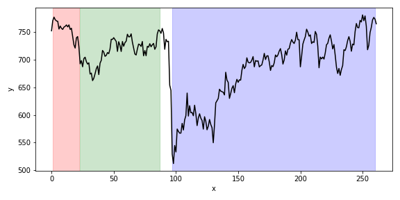
The above example is contrived and easy to solve by more direct means but hopefully it made the approach fairly clear. In this example I apply much the same method but this time to perform a piece-wise isotonic fitting of the FTSE 100 stock index. The graph below shows the last 5 years of the FTSE-100 index at weekly intervals. The segmentation was created by reasoning about random segments just as in the example above, except an Isotonic Regression was fitted instead of a Linear Regression.
The following information was recorded:
segment(Id,Start,Stop,Direction,Fit)I made the following minimal adjustment to the Prolog code:
same_direction(I1,I2) :-
    segment(I1,_,_,G1,_),
    segment(I2,_,_,G2,_),
    G1 = G2.

:- table reach/2.

reach(I1,I2) :-
    same_direction(I1,I2),
    overlap(I1,I2).
reach(I1,I2) :-
    same_direction(I1,X),
    same_direction(X,I2),
    overlap(I1,X),
    reach(X,I2).
I have added the same_direction predicate which requires that the direction of the isotonic regression is the same in overlapping segments for them to be reachable. I have also relaxed the random partitioning condition to a correlation of \(\ge 0.9\). I can now query for the cover as before:
?- find_cover(Cover).which outputs the segmentation in the plot above:
Cover = [(1, 22), (23, 88), (97, 260)].Conclusions
Despite the importance of reasoning in my work, I never made it explicit, nor did I consciously separate it from its subject matter. Adding Prolog to the mix enabled explicit reasoning. A very general modus operandi is to generate facts about your data and reason about them in Prolog. This came natural to me because it is how I work anyway. However, I note that Prolog greatly enhances the possibilities. For example, I would not have pursued the solutions above in practice for lack of easy way to express them. Yet the solutions above are a very direct expression of my intuition regarding what a piece-wise fitting ought to capture, which I would have otherwise compromised on for practical reasons.
The random partitioning technique explained above is one of many broadly applicable ways to generate facts about data. It should be noted that similar methods can be applied to multivariate data and to non-timeseries data with some tweaking. For example, I have a multivariate dataset containing many explanatory variables and one response variable. The coverage across explanatory variables is not uniform in the dataset and I am using Prolog to work out the number and location of the models to be fitted if each model should have explanatory variables in a continuous range. For the subsets of the space which do not have explanatory variable coverage, I am using Prolog to reason about which combination of adjacent models should be used to interpolate the space.
I intend to write more on this topic as I become more experienced with Prolog.