SUMMARY

I show how assumptions about price structure can be used to build a compelling fixed effect (deterministic) price imputation model for the UK residential housing market. The model uses just public price paid data. I describe how the data is collected and processed, how the model is designed, and how it is fitted using the Jax Python package. I showcase some results, I discuss shortcomings and I highlight further necessary work prior to use for decision making under uncertainty.

INTRODUCTION

The UK government publishes price paid data about residential UK property transactions. It contains information like address, sold price and type of property for transactions since 1995. I conjectured that a lot of information about properties must be “priced in” and I wanted to see if I could use just price and address data to impute prices convincingly by making assumptions about the structure of what prices capture.

I’m going to focus on making a fixed effect – deterministic – model although it naturally extends to a mixed effect model by characterising the uncertainty of the residual. The full model is necessary for informed decision making under uncertainty, but the most important and novel component is the fixed effect I’m going to focus on.

All code required to reproduce the analysis is included inline herein.

THE MODEL

I assume that the following assumptions hold in most cases at least locally: (1) residential properties are commensurable and form a single market – i.e. properties are priced relative to each other – and (2) the price ratio of properties are the same over time – i.e. if \(A\) costs twice as much as \(B\) in the past, then it will also in the future. From these I can infer that price ratios are transitive (e.g. if \(A=2B\) and \(B=3C\) then \(A=6C\)) and that the real price of any property can serve as a numeraire for the rest. Abstracting out the numeraire into a latent time varying term \(x_t\), I can express the price of any property as follows: \[p_i^t = \alpha_i x_t\] where \(p^t_i\) is the price of property \(i\) in period \(t\), and \(\alpha_i\) is the latent property specific constant. A “period” is an arbitrary duration, but herein I use calendar months. Note that \(\alpha_i\) is time invariant, and \(x_t\) is period specific. Thus, once \(\alpha_i\) is calculated it can be applied anywhere that \(x_t\) is available to produce the value \(p^t_i\): that is the crux of how the model is able to impute.

The transactions data reveals \(p^t_i\) from which I need to infer \(x_t\) and \(\alpha_i\). This can be formulated as an optimisation problem. Let \(i \in P: P=[1,...,M]\) index each property, let \(t \in T: T=[1,...,T]\) index each period, let \(S_t \subseteq P\) indicate the indexes of properties sold in period \(t\), then:

\[\min_{\alpha_\cdot,x_\cdot}\Bigg[ \sum_{t=1}^T \sum_{s\in S_t} \big( \alpha_s x_t - p^t_s\big)^2\Bigg]\] subject to \(\alpha_s>0\), \(x_t>0\). The optimisation has approximately \(M+T\) degrees of freedom as an upper limit, but the effective degrees of freedom may be lower because the variables are not independent. Further, the final imputation (see implementation section) only uses one of the \(\alpha_i\) set with the rest being nuisance parameters. The function is non-linear, however the within (\(x_t\)) and between (\(\alpha_i\)) period variables keep this problem well behaved in practice by providing constraints on the search space. The inner term of the objective function \((\alpha_s x_t - p^t_s)^2\) has a positive second differential with respect to \(\alpha_i\) and \(x_t\) so its Hessian matrix is positive definite and hence the objective function must be convex.

In the following sections I’ll describe how the data was collected and prepared, and how the model was practically implemented.

DATA COLLECTION AND PREPARATION

The model makes use of two datasets: price paid data and postcode lat/lon data. The former contains property addresses, prices and some basic categorical information whilst the latter contains the latitude and longitude for all UK postal codes. I import both CSVs into a SQLite database for further processing as follows.

I select only postcode, latitude and longitude from the postcodes.csv and pipe it into a SQLite script: loc.sql.

  cat postcodes.csv | \
  cut -d"," -f2,3,4 | \
  sqlite3 --init loc.sql db.sqlite

loc.sql creates a new loc (i.e. location) table and populates it from stdin.

  drop table if exists loc;
  create table loc(pc text, lat float, lon float);
  .mode csv loc
  .import --skip 1 /dev/stdin loc

Similarly, I pick specific columns from the prices.csv data and pipe it into prices.sql.

  cat prices.csv | \
  sed -r 's/","/\t/g' | \
  cut -f2-9 | \
  sqlite3 --init prices.sql db.sqlite

prices.sql creates a temporary prices table and populates it from stdin. It joins the loc table, and then creates a new prices table from the result of the join. It also does a little bit of transformation such as creating a non unique id field to more easily identify specific addresses and converting the lat/lon from degrees to radians.

  drop table if exists prices;
  create temporary table prices_tmp(
  pr float, dt text, pc text, typ text, isnew text,
  dur text, paon text, saon text);
  .mode tabs prices_tmp
  .import /dev/stdin prices_tmp
  
  create table prices as
  select replace(paon||' '||saon||' '||p.pc,'  ',' ') as id,
         radians(lat) as lat, radians(lon) as lon,
         pr, dt, p.pc, typ, isnew, dur, paon, saon
  from prices_tmp p
  inner join loc l on l.pc=p.pc;

The model is built in Python which is not memory efficient so some of the filtering work is done on the SQL side. Namely, I query the database for transactions featuring properties within 2km of a target property. To do this I utilise the added lat/lon. Vanilla SQLite does not have the trigonometric functions required to calculate distance between geographical coordinates, so I register a Python function to handle it:

  import sqlite3
  from math import sin,cos,acos
  
  def great_circle_dist(lat1,lon1,lat2,lon2):
      r1 = sin(lat1)*sin(lat2)
      r2 = cos(lat1)*cos(lat2)*cos(lon2-lon1)
      return 6371 * acos(r1 + r2)
  
  con = sqlite3.connect("db/db.sqlite")
  con.create_function("DIST", 4, great_circle_dist)

I can now define the get_local_by_id function, which returns just those property transactions within 2km of a target property:

  import pandas as pd

  query_id_1km = """
  with
  p0 as (select lat as lat0, lon as lon0, dur
         from prices
         where id='{id}'
         limit 1)
  select p.*, julianday(p.dt) as days
  from prices p join p0
  where p.dur = p0.dur and
        DIST(lat0,lon0,lat,lon) < 2
  order by p.dt;
  """

  def get_local_by_id(id):
      return pd.read_sql_query(
          query_id_1km.format(id=id), con)

In the following section I’ll explain how the data is used to implement a price imputation model.

IMPLEMENTATION

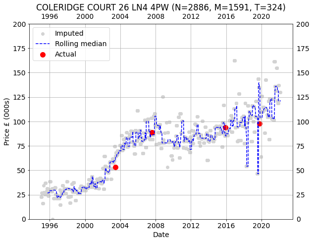
The model focuses on imputing the price for an arbitrary target property. Data is collected from within a 1km radius of the target:

target = "COLERIDGE COURT 26 LN4 4PW"
df     = get_local_by_id(target)

I add a few auxiliary columns to the data-frame. The most important are ym and idx which are integer indexes for the periods and properties respectively.

# Turn calendar months into an index.
df["ym"]  = df["dt"].str.slice(0,7)
ym        = df.ym.unique()
ym        = dict(zip(ym,range(len(ym))))
df["ym"]  = list(map(lambda x: ym[x], df.ym))

# Turn properties into an index.
df.dt     = pd.to_datetime(df.dt)
prop      = df.id.unique()
prop      = dict(zip(prop, range(len(prop))))
df["idx"] = df.id.map(prop)

# Remember the index of the target.
tar_idx   = prop[target]

# Some useful cardinalities for later.
M, N, P   = len(prop), len(df), len(ym)

Since the minimisation problem is convex we can use gradient descent to solve it as a first approximation, for which I use the Python package Jax:

  import numpy as np
  from jax import value_and_grad,jit
  import jax.numpy as jnp

  idx, y, t = df.idx.values, df.pr.values, df.ym.values
  
  def obj(arg, idx, t, y):
      a, p = arg
      return ((a[idx]*p[t]-y)**2).mean()**.5
  
  a = np.random.uniform(1,-1, M)
  p = np.random.uniform(1,-1, P)
  g = jit(value_and_grad(obj))
  
  for _ in range(500000):
      o, (d_a, d_p) = g((a, p), idx, t, y)
      a = jnp.clip(a - 0.25 * d_a, 0)
      p = jnp.clip(p - 0.25 * d_p, 0)

I use RMSE as an objective rather than sum of squares because the numbers involved get very big otherwise which causes Jax to fall over. Note that I clip negative values resulting from a gradient update in order to keep \(a\) and \(p\) positive. Gradient descent takes a large number of iterations to converge, even at high learning rates. It is also sensitive to outliers given that I’m using a least square objective. There are better options than gradient descent for this problem but it will suffice for the proof of concept.

RESULTS

Here are a few pseudo-random examples. The code used to generate the graphs is as follows.

d = df[df.id==target]
y = a[tar_idx]*p[t]/1000
plt.figure(figsize=(9,7))
plt.grid()
plt.scatter(df.dt, y, c="lightgray", label="Imputed")
plt.plot(df.dt, pd.Series(y).rolling(30).median(), c="blue",
         ls="--", label="Rolling median")
plt.scatter(d.dt, d.pr/1000, c="r", s=100, label="Actual")
plt.tick_params(labeltop=True, labelright=True)
plt.xlabel("Date")
plt.ylabel("Price £ (000s)")
plt.title(target)
plt.legend()
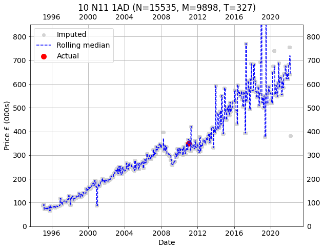
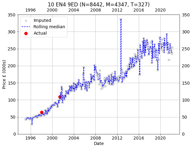
plt.tight_layout()

The gray points are the imputed prices for the target property for every transactions. The red points are actual prices paid for the property. The dashed blue line is a rolling 30 transaction median.

DISCUSSION AND CONCLUSION

The individual imputations tell the same story in the main showing clear trends using just a rolling median. Further, the prices imputed for properties familiar to me are accurate, and this is all prior to any attempts to remove outliers, weighing contributions, perfecting the fitting and so on. For those reasons, I consider this proof of concept a significant success. However, there remain various complications to be addressed:

1. Potentially high degree of freedom – the final imputation uses a property specific \(\alpha_i\) variable and all the \(x_t\) period variables. I.e. roughly \(T\) parameters, with another \(M\) being treated as a nuisance. The model is non-linear and the variables are not independent, so it isn’t entirely clear prima facie how much of a problem the degrees of freedom are. Therefore, the model needs to be cross-validated carefully in both specific and general cases because it is at risk of over-fitting.

2. Random effects – I have considered only a prominent fixed effect but the effort naturally extends into a probabilistic mixed effect model. A search for other fixed effects, and a random effect model is needed (especially given heteroscedasticity of variance) before the model can be used for decision making under uncertainty.

3. Local differences – Different properties have markedly different price series both in terms of shape and variance. Usefully analysing the residual of the fixed effect model may require multiple models in order to take into account the typology of local situations.