SUMMARY

I use lichess.org games data to investigate the extent to which fast thinking is the dominant factor affecting game outcomes at any time control. I show how to (1) frame a pseudo-experiment, (2) database lichess.org data, and (3) carry out the analysis. I argue that fast thinking is most prominent in quick games. I analyse a sample containing games from pairs of users who have played each other at multiple time controls and show that win probabilities established using 180 sec Blitz games are heavily discounted in 600 sec Rapid games. I tentatively conclude that the dominance of fast thinking is significantly reduced at longer time controls.

All code required to replicate the data preparation and analysis is in the post.

INTRODUCTION

I played chess a little bit back when chess.com was a windows app. I picked it up again what must be about 10 months ago at the time of writing (some 20 years later) – as if my life needed another distraction. It initially piqued an interest because I suck at it and wanted to understand why. Kasparov called chess the drosophila of reasoning – perhaps that’s a bit much but it is a rare instance of a scenario involving substantial exercise of your judgement in a fiercely competitive setting that you can repeat ad nauseam and learn from at your own pace.

lichess.org make their games data freely available so I started looking at what could be gleaned about the general happenings in chess games to set a baseline for more personal studies. In this post I investigate whether chess is mostly about fast thinking or whether there is reason to believe that less brute elements of reasoning may also be significantly involved.

HYPOTHESIS AND DESIGN

I want to investigate whether chess involves more than fast thinking for normal chess players. By “fast thinking” I mean any thinking process which is advantageous in chess and which can be employed in short time intervals. For example, trying out possibilities in your head and not making too many mistakes. By this working definition not-fast thinking isn’t applicable in situations requiring speed of execution and I’d venture therefore that fast thinking is more prominent in quicker games. Given pairs of players who have encountered each other at both fast and slower time controls, I aim to investigate the importance of fast thinking by examining to what extent information about the quick games predicts the outcome of the slower games.

There are possibly many ways to conduct this investigation but the one that occurs to me most vividly is to frame the null hypothesis as a counterfactual which can then be pursued as a pseudo-experiment (I’ll explain). The null hypothesis counterfactual (NHC):

NHC: Had there been more time allowed, the outcome would not have been different.

The chess playing population is not homogeneous across time controls. Since I want to compare across time controls I created a homogeneous matched pair sample – detailed in the next section – by considering only games from pairs of players who have played across the time controls I want to test. This given, I can produce a model of win probability using the rating difference between players at the quick time control, and measure how that model changes when it is applied to games in the slower time control. Null Hypothesis (NH):

NH: NHC is true. On average, given some rating difference \(x\), if \(A\) beats \(B\) at the quick time control with a probability \(p\), then \(A\) beats \(B\) at the slower time control with probability \(p' \ge p\).

That is, if fast thinking is the dominant factor determining outcomes in games amongst normal players, it should imply that more time makes the faster thinkers advantage more prominent and the expected outcome more certain. The complementary Alternative Hypothesis (AH):

AH: NHC is false. On average, given some rating difference \(x\), if \(A\) beats \(B\) at the quick time control with a probability \(p\), then \(A\) beats \(B\) at the slower time control with probability \(p' < p\).

In the following sections I’ll describe how the data for this analysis is collected and prepared, and how the analysis itself carried out.

DATA COLLECTION

The lichess.org guys PGN serialise games and make then available for download in bz2 monthly archives. The archives are fairly large – circa 270Gb uncompressed – but we can easily process this without resorting to some Spark based distributed monstrosity. The fields I’ll need for the analysis are: player ids, time control, ratings and result information. I am a fan of the Unix philosophy of using purpose built tools together to achieve bigger tasks, so the whole ETL looks like this:

bzcat march2022.bz2 | \
awk -f parse.awk | \
sqlite3 --init init.sql games.db

bzcat streams the compressed file into a parser which extracts just the bits I need and pipes it into a SQLite database. parse.awk grabs the needed fields and fiddles them a bit so that they occupy less space in the database. E.g. dates as int32, results as int8, and so on.

{
    st = index($0, " ");
    n  = substr($0, 2, st-2);
    v  = substr($0, st+1);
    gsub(/["\]\.]/, "", v)
    x[n] = v;
    if (n == "Termination") {
        tc = x["TimeControl"];
        gsub(/[\+\-]/, ",", tc);
        res = "0";
        if (x["Result"] == "1-0") res="1";
        if (x["Result"] == "0-1") res="-1";
        printf "%s,%s,%s,%s,%s,%s,%s\n",
            x["White"],x["Black"],tc,res,
	    x["UTCDate"],x["WhiteElo"],x["BlackElo"];
        delete x;
    }
}

init.sql creates the games table if it does not exist, flips the read mode to CSV and starts reading stdin into the games table:

create table if not exists games(
    w text, b text, t int, inc int,
    o int, dt int, w_r int, b_r int);
.mode csv games
.import /dev/stdin games

That’s all of it. The March 2022 bz2 imports 91,140,030 games. The final SQLite database for March is about 6.6Gb on disk. If you’re constrained for disk space you can use a compressed virtual ZFS pool to transparently compress the data on the physical volume – then it will be around 1.5Gb on disk.

DATA PREPARATION

The entire preparation of the features for analysis can be expressed as an optional index (for performance) and a single CTE which populates a “features” table.

create index if not exists players_idx 
ON games(w, b);

create table if not exists features as
with

-- Configuration
c as (
  select 180 as lo, 600 as hi),

-- Use pairs over multiple time controls.
g0 as (
  select games.* from games, c
  where t in (lo, hi)),
g1 as (
  select w as p1, b as p2, t from g0
  union all
  select b as p1, w as p2, t from g0),
g2 as (
  select p1, p2 from g1
  group by 1, 2
  having count(distinct t)>1 and p1>p2),
g as (
  select g0.* from g0
  inner join g2 on
    (w=p1 and b=p2) or (w=p2 and b=p1)),

-- User ratings at lowest time control
r0 as (
  select w as p, t, w_r as r from g0
  union all
  select b as p, t, b_r as r from g0),
r as (
  select p, 1.0*sum(r)/count(*) as r
  from r0,c
  where t=lo
  group by 1)

-- Features of interest
select w, b, (r_w.r - r_b.r) as r_diff, g.t, o
from g
join r as r_w on(r_w.p = g.w)
join r as r_b on(r_b.p = g.b);

My fetish for single letter variable names probably isn’t helping you right now, but the CTE is simple. c is a configuration table, it shows that in this instance I’m filtering for user pairs which have played games at 180 and 600 seconds¹. g is the games table which only contains games from user pairs that have played at both 180 and 600 seconds. r is a average user rating table for all users at the lowest time control. The output to the features table are the white player name (w), black player name (b), rating difference at the lowest time control (r_diff), the time allowed (t) and the game outcome (o). The CTE takes about 7.5 minutes to execute on my XPS 13, and yields ~57k games.

ANALYSIS

I start by declaring the few required libraries and I set up a utility function Q which is used to query the SQLite database and return the results.

require(magrittr, quietly=T)
require(dplyr,    quietly=T)
require(mgcv,     quietly=T)

conn <- DBI::dbConnect(
  RSQLite::SQLite(), "data/games.db")
Q <- \(q) DBI::dbFetch(DBI::dbSendQuery(conn, q))

The aim of the analysis is to create a probabilistic model and observe how it differentiates between the 180sec and 600sec time control. A multinomial model is a natural fit and straightforward to carry out using R, but interpretation is a bit trickier, thus for the purpose of exposition I ignore games resulting in a draw so that I can use a binomial model instead. I also ignore spurious games where the difference between the players is 600 points or more. These filters together reduce the ~57k dataset to ~50k. I add to the dataset a dummy variable pos = (r_diff > 0) which indicates whether the rating different is positive or negative – this makes interaction terms easier to interpret.

x <- Q("select * from features
        where abs(r_diff) < 600 and o != 0") %>%
  mutate(o=o==1, t=factor(t), pos=factor(r_diff>0))

I set up a logistical regression with the following formula in R notation:

o ~ r_diff + pos:t -1

The binary outcome o is explained by the rating difference (r_diff) and a set of constants represented by the unpacking of the interaction term pos:t which results in four boolean dummy variables: {t=180,t=600} x {pos=T,pos=F}. The mgcv package adds a constant to formulae automatically and the special instruction -1 removes it.

I execute the model using the mgcv package for General Additive Models (GAMs). GAMs further generalise GLMs (Generalised Linear Models) and are able to take into account significant non-linearities ². I change the basic linear formula slightly prior to execution to subject the r_diff variable to backfitting.

m <- gam(o ~ s(r_diff) + pos:t -1,
  data = x,
  family=binomial,
  method="REML")

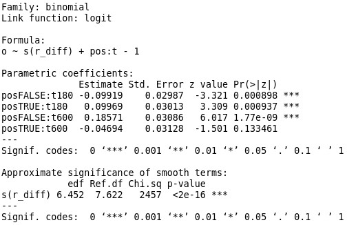
summary(m)
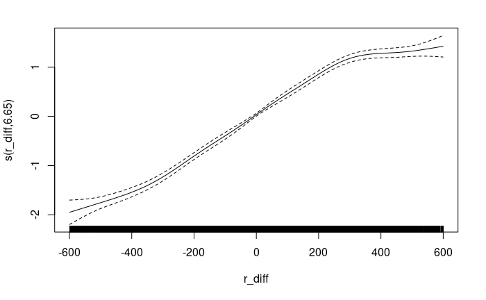
plot(m, pages=F, rug=T, scale=0)

The following diagram shows how the backfitting algorithm re-maps r_diff to a smooth curve prior to ordinary linear regression. Its notably a linear transformation within -300 < r_diff < 300 and departs somewhat at the extrema. The dashed lines indicate the standard error which can be seen to increase with the non-linearity of r_diff.

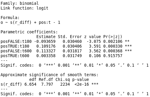
The summary below shows the significance of the backfitted term and the interaction terms. Note that at t=180 the pos=True and pos=False terms are similarly weighted but have contributions in opposite directions as might be expected. That is, on average a lower or higher rating than the opponent results in an decrease or increase in the odds of victory respectively. Note however that it is not the case when t=600. Here, pos=True shows a small and statistically insignificant effect on the odds of victory, whilst pos=False shows a strong (\(e^.113 \approx 1.12\), 12% decreased odds) and statistically significant effect in the opposite direction. That is, whilst in the t=180 case negative rating difference implies an average of \(e^{-.09} \approx .91\) (~9% increase in odds of loss), in the t=600 case the same condition implies a ~12% decrease in odds of loss.

The model has roughly 11 degrees of freedom – mostly in the r_diff smooth – and it fits 50k+ record dataset therefore over-fitting is not a concern. The plot below shows a calibration curve illustrating how predicted probabilities of White victory map to fraction of occurrences: tight!

p <- predict(m, type="response")
x <- seq(0.1, .8, .01)
y <- Map(\(s) {
  cond <- abs(p - s) < .025
  sum(X$o[cond]) / sum(cond)
}, x) %>% unlist

plot(x, y, ylab="Predicted", xlab="Actual")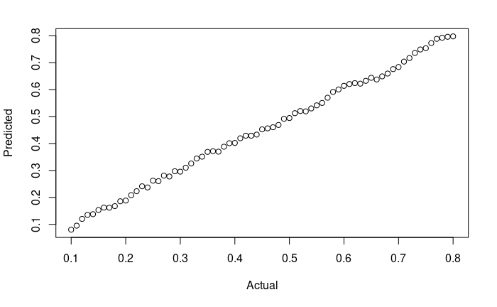

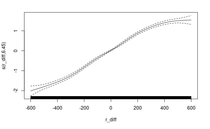
I ran the same analysis on the February 2022 archive. The analysis after filtering includes ~52k games. The r_diff smooth and summary table are presented below and support the same conclusions. At t=600 the interaction term for pos=True is insignificant, but the pos=False term strongly discounts the odds as before except the effect is even stronger compared to the March 2022 archive.